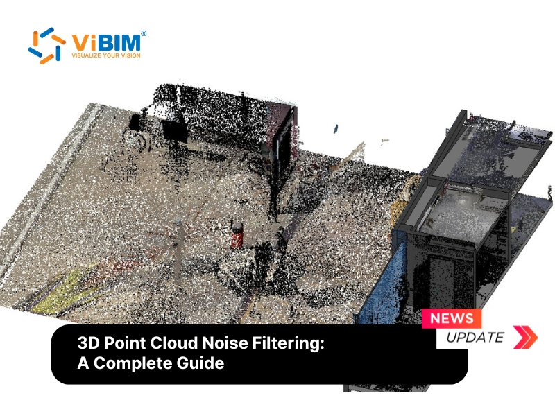
Converting a point cloud into a 3D model means transforming the raw 3D coordinate points of a laser scan or photogrammetry capture into a continuous surface mesh or a vector-based CAD or BIM model. The mesh and the BIM model both count as a 3D model. Point clouds come in several types, including terrestrial laser scans, LiDAR point clouds from mobile or airborne sensors, and photogrammetry point clouds, and the same conversion applies to each.
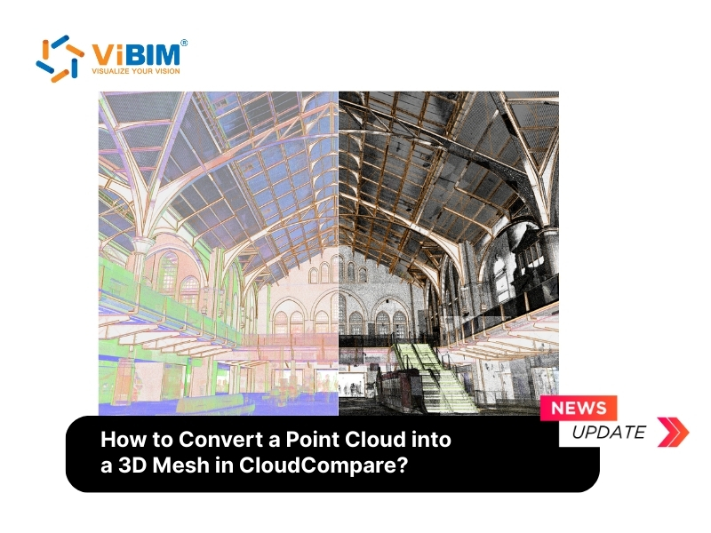
The point cloud to 3D model conversion methods include automated surface reconstruction for a mesh in minutes, manual tracing for a construction-ready BIM model, and AI-assisted platform conversion for large-facility scans that still need a deviation check. The point cloud to 3D model workflow takes a scanned arched hall through five steps in CloudCompare, importing and cleaning the scan, computing normals, generating a Poisson mesh, trimming it by point density, and exporting it to Blender. Common conversion problems include noisy data, which outlier filters remove; oversized files, which subsampling shrinks; misaligned scans, which registration corrects; holes in the mesh, which appear where the scan has no points and close in Blender; and flipped normals, which recomputed orientation fixes.
The sections below then match software to each output, compare a mesh with a BIM model, walk the BIM, Revit, and CAD routes, and set out when an as-built model, several disciplines, or a hard deadline makes outsourcing worth it. The BIM and outsourcing guidance draws on ViBIM’s 1,000+ completed projects since 2014.
Three Methods to Create a 3D Model from a Point Cloud
The three methods to create a 3D model from a point cloud are automated surface reconstruction, manual tracing in CAD or BIM software, and AI-assisted platform conversion. The right method depends on the output you need, how clean the scan is, and which software has to open the result.
A mesh is accepted when its surface stays within tolerance of the original points, while a traced model must also reach the Level of Development (LOD) the project committed to. The input, output, tools, and effort of the three methods are compared below.
| Method | Input needed | Output | Typical tools | Effort |
|---|---|---|---|---|
| Automated surface reconstruction | Clean, subsampled cloud with normals | Polygon mesh (OBJ, STL, PLY) | CloudCompare, MeshLab (Blender for refinement) | Low. Learnable in days, minutes to run |
| Manual tracing in CAD or BIM software | Registered cloud, indexed as RCP/RCS | Parametric BIM model (RVT, IFC) or CAD drawing (DWG) | ReCap, Revit, AutoCAD, SketchUp + Undet | High. Discipline modeling skills, days to weeks |
| AI-assisted platform conversion | Raw or pre-segmented cloud | Simplified CAD or game-ready geometry | Prevu3D | Low to medium. Fast, with simplified geometry |
Automated Surface Reconstruction (Meshing)
Automated surface reconstruction turns the points in a cloud into a continuous polygon mesh with algorithms such as Poisson Surface Reconstruction, Ball Pivoting, or Marching Cubes. CloudCompare runs Poisson reconstruction through a plugin, while MeshLab also offers Ball Pivoting for large, sheet-like datasets. Poisson fits a smooth, watertight surface to the oriented points instead of passing through each one, so it performs best on organic shapes, terrain, and props where slight smoothing is acceptable.
Automated meshing is the fastest way to create a 3D model from a point cloud, and it gives the best result on a scan that has been cleaned and evenly thinned first.
Manual Tracing in CAD or BIM Software
Manual tracing in CAD or BIM software uses the point cloud as a measured reference while a modeler rebuilds each wall, floor, or pipe as clean geometry. Automated meshes come out bumpy on buildings, with flat walls rippling and sharp edges rounding off, so architectural 3D modeling from point clouds is traced instead. Traced in Autodesk Revit BIM software, manual tracing is the only method of the three that produces a construction-ready BIM model. Plugins such as Undet speed up tracing on historic structures and complex interiors where standard shapes do not apply.
AI-Assisted Platform Conversion
AI-assisted platform conversion segments a point cloud into recognizable objects and generates geometry from each segment automatically. AI-assisted platforms such as Prevu3D suit large facilities and digital-twin projects where speed matters more than millimeter fidelity, and where modeling a whole plant by hand would take months.
AI-generated geometry is simplified and still goes through a modeler’s deviation check, and automated segmentation tends to mislabel overlapping equipment and thin structures. A newer research line, the point cloud foundation model, aims to make that segmentation general rather than tool-specific, though nothing production-validated for construction has emerged yet.
Automated surface reconstruction is the method the point cloud to 3D model workflow runs in CloudCompare, from noise removal to Poisson meshing.
Point Cloud to 3D Model Workflow
The point cloud to 3D model workflow is the order in which a raw scan gets cleaned, aligned, given surface normals, reconstructed into a mesh, then trimmed and simplified for use.
The steps work on any laser-scanned 3D point cloud model or photogrammetry scan and turn point cloud data into a 3D model meshed for visualization.
How to convert a point cloud into a 3D model using the open-source software CloudCompare comes down to five steps:
- Import and preprocess the point cloud in CloudCompare
- Compute normals
- Generate a mesh using Poisson Surface Reconstruction
- Clean up and trim the mesh in CloudCompare
- Export from CloudCompare and import to Blender for further editing
Step 1: Import and Preprocess the Point Cloud in CloudCompare
Importing and preprocessing the point cloud in CloudCompare covers loading the file, removing noise and outliers, downsampling the cloud, and aligning the scans when there are several. Poisson reconstruction needs one clean, evenly spaced cloud, so stray points are filtered, dense areas thinned, and separate scans aligned first.
Step 1.1: Launch CloudCompare and import your file
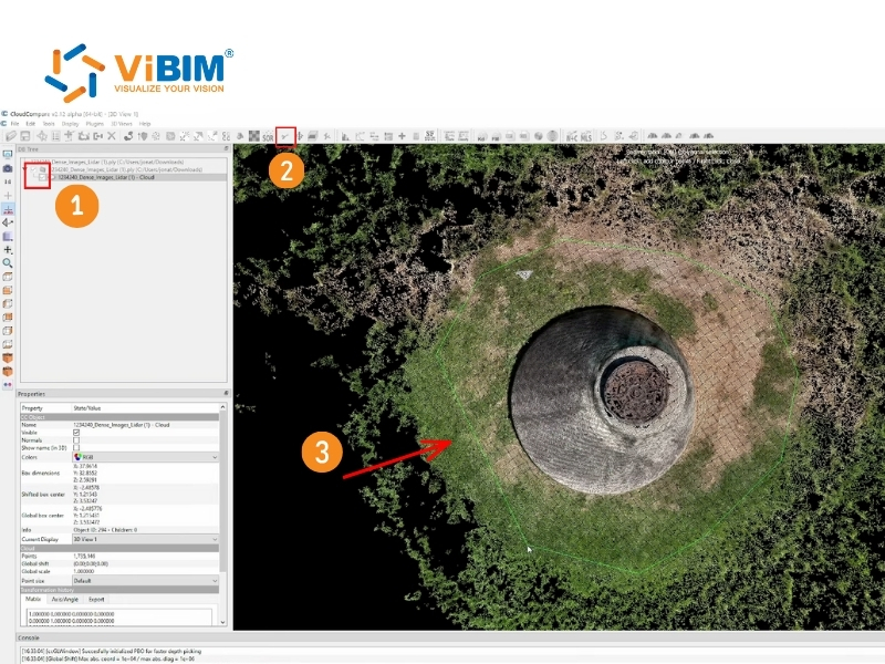
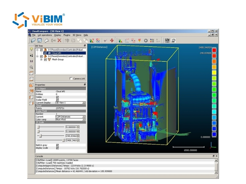
CloudCompare opens PLY, LAS, E57, and XYZ scans directly, but not ReCap RCP or RCS projects. The steps to launch CloudCompare and import a point cloud file are listed below.
- Export any RCP or RCS project to E57 in ReCap before you start.
- Open CloudCompare.
- Go to File > Open and select your point cloud file. Loading may take a few minutes for large files.
- Navigate the scene once the point cloud appears in the 3D view, using the mouse buttons to rotate and pan and the scroll wheel to zoom.
- Accept the “Global Shift” CloudCompare suggests when the file has large coordinates, as georeferenced survey data usually does, because CloudCompare processes data more accurately when coordinates are closer to the origin (0, 0, 0).
Step 1.2: Remove noise and outliers
Noise and outliers in raw scans are mostly ghost points from window reflections, airborne dust, and sensor errors, and the meshing algorithm treats each one as real surface. The steps to remove noise and outliers from a raw scan are listed below.
- Select the point cloud in the DB Tree (left panel) so a yellow outline appears.
- Go to Tools > Clean > SOR filter to remove statistical outliers, keeping the default values for a first pass.
- Go to Tools > Clean > Noise filter if surface noise remains, a second pass of 3D point cloud noise filtering that removes points lying off a locally fitted plane.
- Remove anything the filters missed with Edit > Segment, drawing a polygon around unwanted areas and deleting them.
Step 1.3: Downsample (subsample) to reduce points
High-density clouds (e.g., 50 million points) create computationally heavy meshes, so subsampling reduces the point count while maintaining geometry. Subsampling a dense cloud in CloudCompare takes four actions.
- With the cloud selected, go to Edit > Subsample.
- In the dialog, set “min. space between points” (e.g., 0.01 meters for a building scan), and aim for 500,000 to 1 million points for most cases.
- Click OK, then select the new subsampled cloud in the DB Tree and hide or delete the original to save memory.
- Check the point count in the Properties window (bottom left).
Terrestrial scanners deliver millimeter spacing, so a 0.01 m setting removes most of the points and still keeps walls and floors intact. A LiDAR point cloud to 3D model project starts from different input, since airborne sensors capture points tens of centimeters apart, already georeferenced and often classified into ground and vegetation, so subsampling has far less to remove.
Step 1.4: Align if multiple clouds (optional)
Aligning multiple clouds through registration puts separate scans into one coordinate system, so Poisson reconstruction reads them as one surface instead of several offset copies. Aligning and merging two scans in CloudCompare takes five actions.
- Select both point clouds, one as the reference and one to align.
- Go to Tools > Registration > Align (point pairs picking) and pick at least three matching points in each cloud for a rough alignment.
- Run Fine registration (ICP) from the same menu to refine the fit.
- Confirm the RMS (Root Mean Square) error is low before you continue.
- Go to Edit > Merge to combine the aligned clouds into one.
Step 2: Compute Normals
You must compute normals, vectors perpendicular to the surface, before generating a mesh, because the mesh uses them to decide which side of each polygon faces out. Raw point clouds typically lack this orientation data. Computing normals on the subsampled cloud takes six actions in CloudCompare.
- Select the subsampled point cloud.
- Go to Edit > Normals > Compute.
- Select the Surface approximation method that matches the geometry.
- Plane: The plane method fits flat surfaces such as walls and floors and tolerates noise, but it rounds off sharp edges and corners.
- Triangulation: The triangulation method keeps sharp edges but reacts badly to noise.
- Quadric: The quadric method fits curved architectural features such as vaults and arches.
- Set the Radius, the local neighborhood used to calculate each normal, to Auto or 5 to 10 times your subsample spacing (e.g., 0.05 to 0.1 m), since a larger radius smooths normals but may round off sharp corners.
- Set Orientation to “Minimum Spanning Tree” (MST) with a KNN (K-Nearest Neighbors) value of 10 to 20 so orientation stays consistent across the model.
- Click OK, and the point cloud changes appearance to show shading based on lighting direction.
Step 3: Generate a Mesh Using Poisson Surface Reconstruction
Generating a mesh using Poisson Surface Reconstruction takes the cloud with computed normals as input and returns a watertight mesh plus a density scalar field for trimming. A watertight mesh encloses a volume, which solid models and 3D prints need. The steps to generate a mesh with the PoissonRecon plugin are listed below.
- Select the point cloud that contains your computed normals in the DB Tree (left panel) so the plugin uses the correct input data.
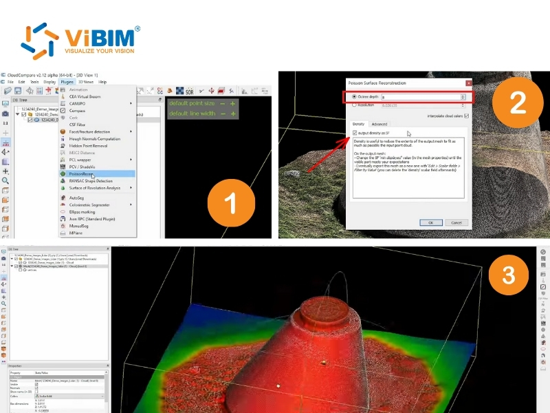
- Open the Plugins menu and choose PoissonRecon.
- Set the Octree depth between 8 and 12, since higher values yield more detail but significantly increase processing time.
- Check “Output density as SF” so the software generates a scalar field you can use for trimming later.
- Optionally, raise Samples per node above its default of 1.5 when the cloud is noisy, since higher values produce a smoother surface.
- Click OK and wait a few minutes for the new mesh to appear in the DB Tree.
The checks to run on the new mesh and its density scalar field are listed below.
- Mesh display: The new mesh appears in the 3D view as a triangular surface, often in a default gray shade with basic shading.
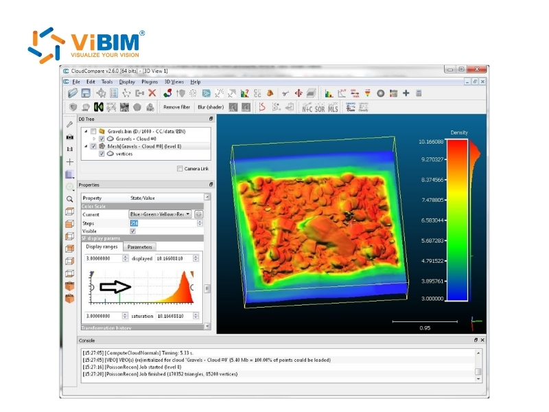
- Density color map: Switch to the density SF in the Properties window (bottom left) under SF display params to apply a color map, and adjust the ramp through the histogram graph if you need a different scale.
- Red and yellow areas: Red and yellow mark high-density areas, where the data is most reliable and accurate.
- Blue and green areas: Blue and green mark low-density zones, often noise or extrapolated geometry that Step 4 removes.
- Failed run: A run that fails, usually from missing normals or insufficient RAM, shows an error message, and the fix is to recheck the normals and try a lower octree depth.
Step 4: Clean Up and Trim the Mesh in CloudCompare
Cleaning up and trimming the mesh in CloudCompare removes extrapolated geometry that does not belong to the scanned object, using the density scalar field from Step 3 to find it. Trimming the reconstructed mesh takes six actions.
- Select the newly created mesh in the DB Tree.
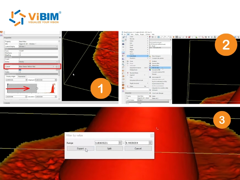
- In the Color Scale section of the Properties panel, set the ramp to Blue, Green, Yellow, and Red.
- Drag the lower threshold slider until only the dense yellow and red regions remain visible in the viewport.
- Go to Edit > Scalar Fields > Filter by Value, using the current range from the SF display parameters so the filter matches exactly what you see on the screen.
- Click Split to generate two separate meshes, one with the kept polygons and one with the discarded noise.
- Delete the mesh containing the unwanted parts, and keep the clean version, such as “mesh.part”, for further processing.
Step 5: Export from CloudCompare and Import to Blender for Further Editing
Exporting the mesh from CloudCompare and importing it into Blender moves the model into software built for sculpting, hole filling, decimation, and retopology. The steps to export the mesh and import it into Blender are listed below.
- Select the final mesh in the DB Tree.
- Go to File > Save to export the object.
- Choose the file format for the next tool, .PLY to keep the vertex colors a Poisson mesh inherits from a colored cloud, .STL for 3D printing, or .OBJ when the target software requires it, since CloudCompare writes OBJ vertices without color.
- Open Blender and delete the default cube by selecting it, pressing X, and confirming Delete.
- Go to File > Import and select Wavefront (.obj), or the matching option for your format.
- Press Tab to switch to Edit Mode and work on the geometry directly.
The Blender tools that refine an imported mesh are listed below.
- Sculpt Mode: Smooth out rough patches in the surface.
- Decimate Modifier: Reduce the polygon count when the mesh is too heavy for your downstream software.
- Fill with the F key: Select the open edges around a hole and press F to close it.
- Vertex colors to UV textures: Vertex colors import differently from standard image maps, so bake them to a UV texture before texturing.
- Retopology add-ons: Run a tool such as Quad Remesher when the model is intended for animation or game engines.
To understand the process more easily, watch this video:
Not every scan goes from point cloud to 3D model cleanly on the first pass.
Common Problems When Converting Point Clouds to 3D Models
Five common problems when converting point clouds to 3D models are noisy data, oversized files, misaligned scans, holes in the mesh, and flipped normals.
The causes and fixes of common point cloud to 3D model problems are listed below.
- Noisy data: Reflections from glass, dust, and moving objects leave stray points that warp the surface. Run the SOR and noise filters from Step 1.2 before meshing.
- Oversized files: Poisson reconstruction on an unthinned scan can run a workstation out of RAM. Subsample first (Step 1.3), and when scans move between teams, split them into RCS files of 5 GB or less, the size we ask clients to send.
- Misaligned scans: Scans merged without registration leave doubled walls and layered floors in the mesh. Align them with point pairs and ICP (Step 1.4) before merging.
- Holes in the mesh: Areas the scanner never reached leave gaps with no points, and Poisson bridges them with invented surface that density trimming (Step 4) removes again. Close the openings you need in Blender (Step 5).
- Flipped normals: Inconsistent normals make the mesh render patchy, with holes or inverted faces. Recompute normals with MST orientation (Step 2) and check the shading before you reconstruct.
Each of these fixes runs in software, and the tools differ in what they produce.
Which Software Converts a Point Cloud into a 3D Model?
Software that converts a point cloud into a 3D model falls into three groups, free mesh tools such as CloudCompare and MeshLab, commercial platforms such as Agisoft Metashape, Autodesk ReCap, and Revit, and AI-assisted converters such as Prevu3D.
The point cloud to 3D model software named most often, and the file format or model each one produces, are listed below.
- CloudCompare: CloudCompare cleans, subsamples, and meshes a point cloud, runs every step of the point cloud to 3D model workflow, and exports OBJ, STL, or PLY meshes.
- MeshLab: MeshLab reconstructs and repairs meshes with Ball Pivoting and Poisson filters and exports the same mesh formats.
- Agisoft Metashape: Metashape builds textured meshes from photos or dense point clouds on a paid license.
- Autodesk ReCap: ReCap registers raw scans and indexes them into RCP or RCS files for Autodesk tools.
- Revit and Archicad: Modelers trace the indexed cloud in Revit or Archicad into parametric BIM models in RVT or IFC, the two authoring tools compared among the best scan to BIM software.
- Prevu3D: Prevu3D segments a scan into objects and returns simplified geometry for digital twins.
Can You Convert a Point Cloud to a 3D Model for Free?
Yes, you can convert a point cloud to a 3D model for free, because the open-source tools CloudCompare, MeshLab, and Blender cover import, cleanup, meshing, and export. The free route ends at the mesh for most jobs, since an RVT deliverable needs a commercial Revit license and the modeling skill to drive it.
Should You Convert Your Point Cloud to a Mesh or a BIM Model?
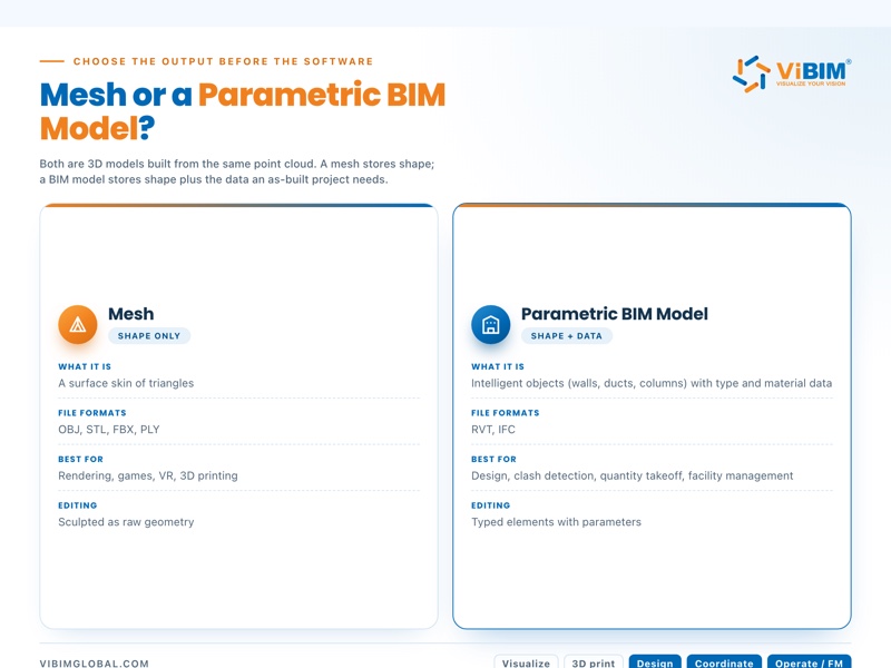
You should convert your point cloud to a mesh when you need geometry for visualization, games, or web viewers, to a BIM model when the geometry must hold wall types and asset data for as-built documentation, renovation, or facility management, and to CAD linework when only 2D drawings are needed.
The differences between a mesh and a parametric BIM model are compared below.
| Mesh | Parametric BIM model | |
|---|---|---|
| What it is | A surface skin of triangles | Intelligent objects (walls, ducts, columns) with type and material data |
| File formats | OBJ, STL, FBX, PLY | RVT, IFC |
| Downstream use | Rendering, games, VR, 3D printing | Design, clash detection, quantity takeoff, facility management |
| Editing | Sculpted as raw geometry | Edited as typed elements with parameters |
A mesh stores shape only, so it can look photorealistic and still answer none of the questions an as-built project asks, such as what a wall is made of or which duct feeds which room. The point cloud vs mesh comparison draws the same line one step earlier, between the raw scan and its surface. A BIM model built from a scan usually lands at LOD 200 to 300 for as-built work, and scan density decides whether it can go further, since mobile-scan data often caps the whole model at LOD 300.
The same cleaned cloud can be traced into a BIM model, a Revit model, or CAD linework.
How to Convert a Point Cloud to a BIM Model
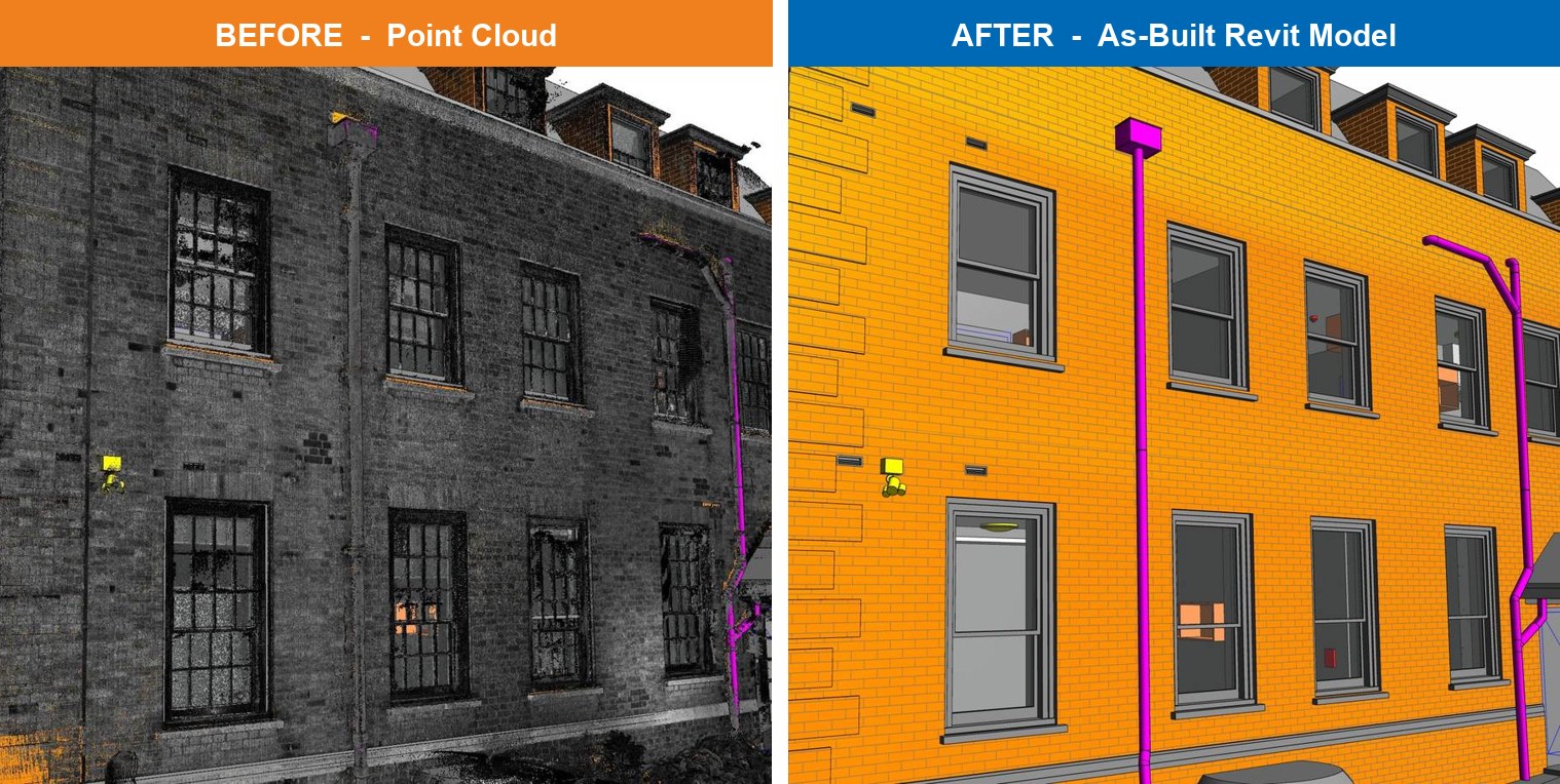
You convert a point cloud to a BIM model by registering and indexing the scan, then tracing each discipline over it as parametric elements. BIM modeling with point clouds usually runs architecture first, then structure, then MEP, and closes with a QC check against the scan.
Can You Build a Revit Model from a Point Cloud?
Yes, you can build a Revit model from a point cloud, but Revit reconstructs no surface on its own, so each wall, floor, structural member, and MEP run is traced by hand as a native family. Revit links the scan through Insert > Point Cloud and reads only ReCap RCP or RCS files, so raw E57 or LAS data is indexed in ReCap first. A Revit point cloud stays a linked reference, so modelers set section boxes and view ranges to trace one level at a time.
How to Convert Point Clouds to CAD Files
You convert point clouds to CAD files by tracing the scan into 2D vector linework and exporting it to as-built drawings, floor plans, site plans, or sections. The three steps that turn a point cloud into CAD linework are listed below.
- Index the scan in ReCap and attach it in AutoCAD or Civil 3D as an underlay.
- Snap lines, polylines, and arcs to wall edges, corners, and floor levels in the cloud.
- Export the drawing to DWG or the CAD format your team works in.
Linework holds no wall types or materials, so a CAD to BIM conversion is the usual next step once the drawing needs them.
When Should You Outsource Point Cloud to 3D Model Conversion?
You should outsource point cloud to 3D model conversion when the deliverable is an as-built BIM model, spans multiple disciplines, or runs against a hard deadline, and you should do it yourself when you only need a mesh from a small, clean scan.
The criteria that separate a DIY job from an outsourced one are listed below.
| Criteria | DIY makes sense | Outsourcing makes sense |
|---|---|---|
| Output | Visual mesh | Parametric BIM model (RVT, IFC) |
| Data size | A single, clean scan on one workstation | Multi-scan projects across floors or buildings |
| Scope | One visual shell, no disciplines | Architecture, structure, and MEP |
| QC | Visual self-check | Deviation check against the cloud |
| Deadline | Flexible | Fixed handover dates |
Output and QC are the two criteria one person rarely covers alone, because a BIM model needs discipline modeling skill and a deviation check needs a second reviewer. ViBIM’s delivery process is built around those two criteria.
How ViBIM Delivers BIM Models from Point Clouds
ViBIM delivers BIM models from point clouds in three phases, scoping the scan before a quote, modeling each discipline in Revit to the agreed LOD, and checking the model before handover. ViBIM’s commercial point cloud modeling services take RCP, RCS, or E57 scans and return RVT, IFC, or DWG files.
The standards and terms behind how ViBIM delivers BIM models are listed below.
- Two independent QC layers: Each model is checked for geometry, parameters, deviation from the cloud, missing elements, and data consistency.
- BIM Forum LOD and ISO 19650: Models are delivered from LOD 200 to LOD 500 and are compatible with ISO 19650.
- 99% on-time delivery: ViBIM has met the agreed deadline on 99% of its projects for clients in the UK, Canada, the USA, Australia, and the EU.
- Quotes within 12 to 24 hours: Each quote sets out the scope of work, timeline, and pricing.
- Dedicated project manager: One project manager runs each job, and typical projects take one to three weeks.
- Free trial project: A new client can run one project free to calibrate the QC standard before committing.
Send your point cloud or project brief to ViBIM to get a scoped quote, from a single floor to a full building under ViBIM’s Revit modeling outsourcing services. If the scan is not ready yet, site photos, existing 2D drawings, or LGS TrueView files are enough for a preliminary estimate.
Vietnam BIM Consultancy and Technology Application Company Limited (ViBIM)
- Headquarters: 10th floor, CIT Building, No 6, Alley 15, Duy Tan street, Cau Giay ward, Hanoi, Vietnam
- Phone: +84 944 798 298
- Email: info@vibim.com.vn